Rewriting Ouija in PyMC3

Ouija ¹ is a trajectory inference tool that recovers the pseudotimes of cells in a scRNA-seq dataset. Rather than fitting a curve or graph through the cells in a reduced dimensional space, Ouija does parameteric curve fitting on a handful of genes. Namely, a gene can be fitted as switch-like or transiently activated:

The main advantage is that the inferred parameters are interpretable.

Ouija is a bayesian generative model written in the probabilistic programming language Stan. I personally prefer PyMC3, mainly because of my comfort with the Python language. This post documents my attempt at converting the Ouija model to PyMC3 for learning purposes, and to potentially build on it with new features.

Ouija model

The noise model in Ouija is a zero-inflated Student’s t-distribution. Zero-inflation in scRNA-seq is due to the log transformation applied to normalize the data.² UMI counts are not actually zero-inflated ³ and a negative binomial or poisson distribution should be able to accurately model the error. However, this is a recent topic of discussion, therefore many methods prior to this relied on a log-transformation to make the count data approximately normal, Ouija being no exception.

The error model is as follows:

\[\label{eq:noisemodel} \begin{equation} y_{ng} \sim ZIStudentT_{\nu}(\pi_{ng}, \mu_{ng}, \sigma^2_{ng}) \\ \sigma^2_{ng} = (1 + \phi)\mu_{ng} + \epsilon \\ \pi_{ng} \sim Bernoulli(logit^{-1}(\beta_0 + \beta_1 \mu_{ng})) \\ \mu_{ng} = \mu(t_n, \Theta_g) \\ \beta_0, \beta_1 \sim Normal(0, 0.1) \\ \phi \sim Gamma(\alpha_{\phi}, \beta_{\phi}) \\ \end{equation}\]

We start from the top. Line 1 gives us the model likelihood for gene $g$ in cell $n$, which in this case is a zero-inflated t-distribution with known degrees-of-freedom $\nu$, set by default to 10. The remaining parameters of the zero-inflated t-distribution are:

• $\mu$: The mean of the distribution. Line 4 shows that this is calculated based on the parameteric form of the gene (switch-like or transient), which is a function of the cell’s pseudotime $t_n$ and the gene specific parameters $\Theta_g$.
• $\sigma$: The scale parameter. In normalized RNA-seq counts the variance for gene is related to its mean using the parametric form shown in line 2. This takes overdispersion into account. You can find more discussion on this in the supplementary text of the Ouija paper ¹.
• $\pi$: The probability of a zero. Line 3 tells us that this probability is estimated as a linear model with the mean as the covariate. Indeed we observe less zeros in more abundant genes, and therefore expect a negative relationship between a gene’s mean expression and its dropout rate.

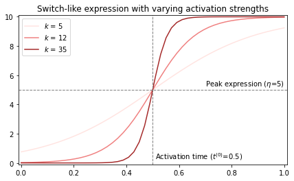
As mentioned, the function $\mu(t_n, \Theta_g)$ gives us the expected expression of a gene (ignoring dropout) at a particular pseudotime $t$. There are two such functions. The switch-like function is defined as follows:

\[\label{eq:switchmodel} \begin{equation} \mu(t_n, \Theta_g) = \frac{2\eta}{1 + exp(-k_g(t_n - t_g^{(0)}))} \\ \eta_g \sim Gamma(\delta/2, 1/2) \\ k_g \sim Normal(\mu_g^{(k)}, 1 / \tau_g^{(k)}) \\ t_g^{(0)} \sim TruncNorm_{[0, 1)}(\mu_g^{(t)}, 1 / \tau_g^{(t)}) \end{equation}\]

The base of the function is a sigmoid, i.e. $f(t) = \frac{1}{1 + exp(-t)}$. The three parameters define different aspects of the sigmoid, namely the peak expression ($\eta$), the activation strength ($k$), and the activation time ($t^{(0)}$). All parameters of the prior distributions are user-specified, save for $\delta$, which is a parameter with its own prior that needs to be inferred as well. We will see this come back later in the code. The default parameters are diffuse: $k \sim Normal(0, 5)$ and $t \sim TruncNorm_{[0, 1)}(0.5, 1)$.

Below figure shows how we can think about the parameters, although later we will plot the prior predictives to get a better feel for the effect of the prior distributions.

The transient function has the classic Gaussian shape:

\[\label{eq:transientmodel} \begin{equation} \mu(t_n, \Theta_g) = 2 \eta_g exp(- \lambda b_g (t_n - p_g)^2) \\ \eta_g \sim Gamma(\delta/2, 1/2) \\ b_g \sim TruncNorm_{[0, \inf)}(\mu_g^{(b)}, 1/\tau_g^{(b)}) \\ p_g \sim TruncNorm_{[0, 1)}(\mu_g^{(p)}, 1/\tau_g^{(p)}) \end{equation}\]

The base function is a bell curve: $f(t) = exp(-t^2)$. The parameters are analogous to the switch-like model. Again $\eta$ denotes the expression at the peak of the curve, and $p$ the activation time. The analagous parameter for activation strength is the activation length $b$, i.e. the duration of transient expression of the gene. Default parameters are $b \sim TruncNorm_{[0, \inf)}(50, 10)$ and $p \sim TruncNorm_{[0, 1)}(0.5, 0.1)$.

We can again visualize the shape:

Zero-inflated Student’s t-distribution

PyMC3 does not come equiped with a zero-inflated t-distribution. However we can peak inside the ZeroInflatedPoisson class to see how we can implement such a distribution. Based on this I find that I need to define three class methods: the __init__() constructor, which takes the model’s parameters as input; random() which returns random samples from the distribution; and logp() which, given a value in the domain of the distribution, returns its log-probability.

Implementing the constructor is straightforward. However we should be aware that the parameters can potentially be pm.Distributions themselves. Remember that the distribution we’re implementing now is the model’s likelihood, and in a bayesian setting the parameters of this likelihood have priors, and will therefore be distributions themselves. Also even when the distribution doesn’t represent the likelihood, parameters of priors can too have distributions (hyperpriors). We thus make sure that the parameters are Theano tensor variables:

class ZeroInflatedStudentT(pm.Continuous):
    def __init__(self, nu, mu, sigma, pi, *args, **kwargs):
        super(ZeroInflatedStudentT, self).__init__(*args, **kwargs)
        self.nu = tt.as_tensor_variable(pm.floatX(nu))
        self.mu = tt.as_tensor_variable(mu)
        lam, sigma = pm.distributions.continuous.get_tau_sigma(tau=None, sigma=sigma)
        self.lam = lam = tt.as_tensor_variable(lam)
        self.sigma = sigma = tt.as_tensor_variable(sigma)
        self.pi = pi = tt.as_tensor_variable(pm.floatX(pi))
        self.studentT = pm.StudentT.dist(nu, mu, lam=lam)

Next is the random() method. To sample from a zero-inflated model, we can think generatively. First we sample from the base distribution - in this case the t-distribution. We then draw from a bernoulli distribution, and return our base distribution sample if the bernoulli sample equals 1. If not we return a zero. If the $p$ parameter of the bernoulli is 1, we are always returning the sample from the base distribution and have effectively removed the zero-inflation. As $p$ gets closer to zero, we progressively expect to find more zeros as we sample from the distribution. The $\pi$ parameter of this model does exactly that.

This generative thinking is reflected in the code. We first sample from the distributions of the parameters (L2-4), and use those values to sample from the t-distribution (L5-7). We use the sampled values of pi to determine if the method should return a zero or the sample of the t-distribution (L8).

    def random(self, point=None, size=None):
        nu, mu, lam, pi = pm.distributions.draw_values(
            [self.nu, self.mu, self.lam, self.pi], 
            point=point, size=size)
        g = pm.distributions.generate_samples(
            sp.stats.t.rvs, nu, loc=mu, scale=lam**-0.5, 
            dist_shape=self.shape, size=size)
        return g * (np.random.random(g.shape) < (1 - pi))

Finally we define the logp() method. When we encouter a zero, i.e. $y=0$, this could be due to the zero-inflation process or simply because the gene was not expressed. The probability of a zero is therefore the sum of both events. However when $y \neq 0$, the probability is only dependent on the likelihood (weighted by the probability of not encoutering a dropout):

\[\label{eq:dropout} \begin{equation} P(y \vert p, \theta) = \begin{cases} P_{dropout}(1 \vert p) + P_{dropout}(0 \vert p)P_{likelihood}(y \vert \theta), & \text{if } y = 0 \\ P_{dropout}(0 \vert p)P_{likelihood}(y \vert \theta), & \text{otherwise} \end{cases} \end{equation}\]

Using theano’s tt.switch we can define such a conditional likelhood:

    def logp(self, value):
        logp_val = tt.switch(
            tt.neq(value, 0),
            tt.log1p(-self.pi) + self.studentT.logp(value),
            pm.logaddexp(tt.log(self.pi), tt.log1p(-self.pi) + self.studentT.logp(0)))
        return logp_val

We work with log-probabilities due to reasons related to numerical stabillity. Therefore, addition of log-probabilities translates to multiplication of probabilities, and this what we see in line 4, which translates to the $y \neq 0$ case in formula $\eqref{eq:dropout}$ above. When we want to take the sum of the actual probabilities, we can make use of the convenience function pm.logaddexp, which as the name implies converts the log-probabilities back to probabilities using the exponential function, sums them up, and subsequantly log-transforms them back again (L5).

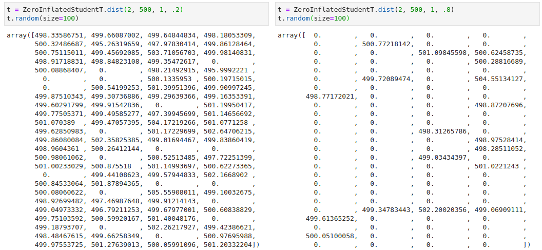
With this, we can test out our new distribution. First we do a simply to check to see if varying the pi parameter indeed changes the number of zeros in our data:

We then generate a simple dataset using this distribution and see if PyMC3 can accurately infer the parameters.

n = 300
prob_dropout = 0.3
mean_expr = 5
scale_expr = 3
dof = 2
dropouts = np.random.binomial(1, prob_dropout, size=n)
expr = (1 - dropouts) * sp.stats.t.rvs(df=dof, loc=mean_expr, 
                                       scale=scale_expr, size=n)
plt.hist(expr, bins=50);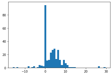

Our model is simple:

with pm.Model() as t_model:
    p = pm.Normal('p', 0, 1.5)
    pi = pm.Deterministic('pi', pm.math.invlogit(p))
    mu = pm.Normal('mu', 0, 10)
    sigma = pm.Exponential('sigma', .5)
    nu = pm.Gamma('nu', alpha=5, beta=2)
    obs = ZeroInflatedStudentT('obs', nu=nu, mu=mu, sigma=sigma, 
                               pi=pi, observed=expr)

We have our ZeroInflatedStudentT likelihood at the bottom, where we pass in our generated data in the observed parameter. We use a gamma distribution for nu, the degrees of freedom parameter, as its flexibility allows us to put little probability mass at small values, where the tails are extremely heavy and extreme values become plausible. In general we know this not to be the case and thus encode this in our prior. We use a logit link function to transform the p parameter to be between 0 and 1, as the pi parameter of the zero-inflated model represents a probability. The standard deviation for p is delibarately chosen to be 1.5, so that we can get a uniform distribution over the probability space. Lower values will concentrate the mass at 0.5, and higher values will push the mass to 0 and 1.

In general it is a good exercise to plot the implications of our priors using prior predictive sampling. We will do that more extensively with the final Ouija model. For now we just plot the prior distributions themselves.

with t_model:
    priorpred = pm.sample_prior_predictive()

fig, axs = plt.subplots(figsize=(12, 3), ncols=5)
axs[0].hist(priorpred['pi'], bins=20); axs[0].set_title('pi')
axs[1].hist(priorpred['mu'], bins=20); axs[1].set_title('mu')
axs[2].hist(priorpred['sigma'], bins=20); axs[2].set_title('sigma')
axs[3].hist(priorpred['nu'], bins=20); axs[3].set_title('nu')
axs[4].hist(priorpred['obs']); axs[4].set_title('obs')
fig.tight_layout()

We sample without problems and find the estimated parameters to be accurate:

with t_model:
    trace = pm.sample()

lines = {'pi': prob_dropout, 'mu': mean_expr, 
         'sigma': scale_expr, 'nu': dof}
pm.traceplot(trace, lines=[[k, {}, v] for k, v in lines.items()]);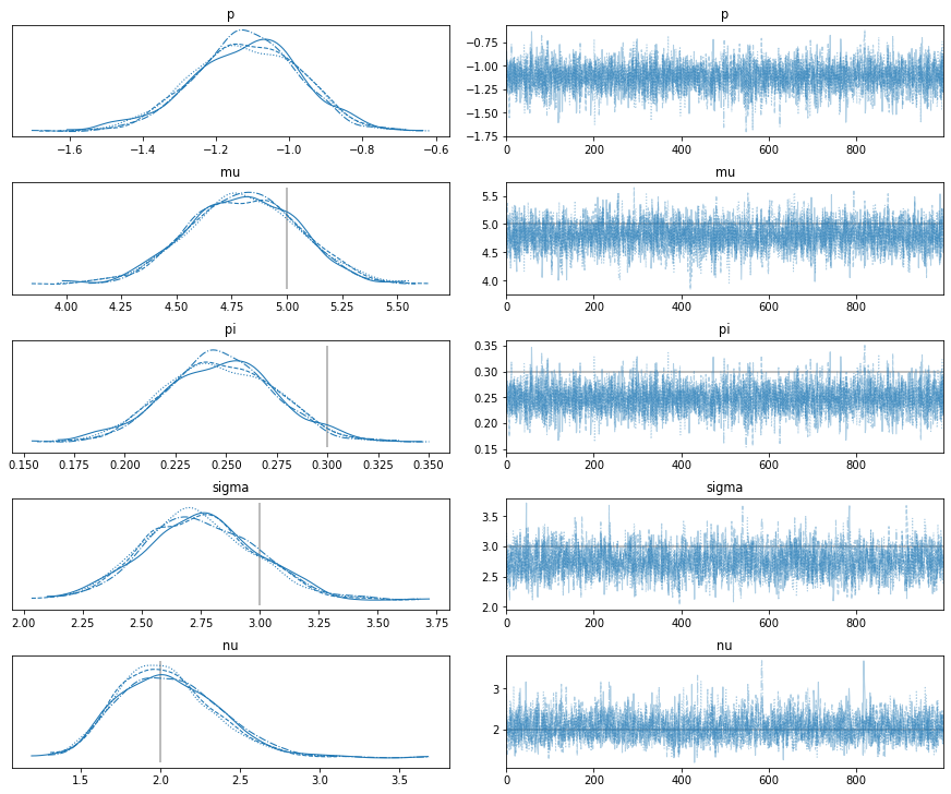

Ouija in PyMC3

We start building the Ouija Stan model in PyMC3. Let’s look at how the likelihood looks like for the switch-like genes in Stan. I will omit lines of code that are not related.

data {
  int<lower = 2> N; // number of cells
  int<lower = 0> G_switch; // number of switch-like genes
  ...
  vector<lower = 0>[N] Y_switch[G_switch]; // matrix of gene expression values
  ...
  real student_df; // student d-o-f
}

parameters {
    ...
    real beta[2];
}

model {
  ...
  beta ~ normal(0, 0.1);
  ...
  // Switch likelihood
  for(g in 1:G_switch) {
    for(i in 1:N) {
      if(Y_switch[g][i] == 0) {
        target += log_sum_exp(bernoulli_logit_lpmf(1 | beta[1] + beta[2] * mu_switch[g][i]),
                              bernoulli_logit_lpmf(0 | beta[1] + beta[2] * mu_switch[g][i]) + 
                              student_t_lpdf(Y_switch[g][i] | student_df, mu_switch[g][i], sd_switch[g][i]));
      } else {
        target += bernoulli_logit_lpmf(0 | beta[1] + beta[2] * mu_switch[g][i]) + 
        student_t_lpdf(Y_switch[g][i] | student_df, mu_switch[g][i], sd_switch[g][i]);
      }
    }
  }
  ...
}

In the data block there are the known values, namely the number of cells and genes, the data itself, and the pre-specified degrees-of-freedom parameter $\nu$ for the Student’s T likelihood. In the model block there is a double for-loop that iterates through the G_switch switch-like genes and N cells. Within the nested for-loop, the zero-inflation is handled in a similar fashion as describe before using a Bernoulli dropout. As defined in $\eqref{eq:noisemodel}$, the dropout probability is trained using a linear model with the gene’s expected expression as the covariate. The beta coefficients are defined in the parameters block and assigned a prior distribution in the model block.

We start writing our model in PyMC by translating the above:

Y_switch = Y.loc[:, response_type == 'switch']
N, P_switch = Y_switch.shape

with pm.Model() as ouija:
    # Dropout
    beta = pm.Normal('beta', 0, 0.1, shape=2)
    pi_switch = pm.math.invlogit(beta[0] + beta[1] * mu_switch)

    # Switch likelihood
    for p in range(P_switch):
        ZeroInflatedStudentT(f'switch_{p}', nu=student_df, 
                             mu=mu_switch[:, p], sigma=std_switch[:, p], 
                             pi=pi_switch[:, p], observed=Y_switch.iloc[:, p])

The translation is relatively straight-forward. We don’t need a double for-loop as everything is vectorized within PyMC. Next we look at how the mean mean_switch and the standard deviation sd_switch are constructed using their specific parametric forms shown in equations $\eqref{eq:noisemodel}$ and $\eqref{eq:switchmodel}$.

data {
  real k_means[G_switch]; // mean parameters for k provided by user
  real<lower = 0> k_sd[G_switch]; // standard deviation parameters for k provided by user
  
  real t0_means[G_switch]; // mean parameters for t0 provided by user
  real<lower = 0> t0_sd[G_switch]; // standard deviation parameters for t0 provided by user
}

parameters {
  // mean-variance "overdispersion" parameter 
  real<lower = 0> phi; 
  
  // switch parameters
  real k[G_switch];
  real<lower = 0, upper = 1> t0[G_switch];
  real<lower = 0> mu0_switch[G_switch];
}

transformed parameters {
  vector[N] mu_switch[G_switch]; 
  vector<lower = 0>[N] sd_switch[G_switch];
  ...

  for(g in 1:G_switch) {
    for(i in 1:N) {
      mu_switch[g][i] = 2 * mu0_switch[g] / (1 + exp(-k[g] * (t[i] - t0[g])));
      sd_switch[g][i] = sqrt( (1 + phi) * mu_switch[g][i] + 0.01);
    }
  }
  ...
}

model {
  k ~ normal(k_means, k_sd);
  t0 ~ normal(t0_means, t0_sd);
  mu0_switch ~ gamma(mu_hyper / 2, 0.5);
  phi ~ gamma(12, 4); 
  ...
}

Again, the parameters that have to be inferred are declared in the parameters block. For modeling the mean, these are the peak expression mu0_switch, activation strength k, and activation time t0. For the variance there is the overdispersion parameter phi. These all come together to calculate the mean and variance for each gene in each cell in the transformed parameters block. In the model block we can see that the latter two mean parameters are defined as normal distributions with user-specified hyperpriors for the means and variances. Conversely, the mu_hyper value in the expression peaks mu0_switch is a parameter that has to be trained rather than a user-specified hyperprior, effectively inducing shrinkage of the expression peaks towards the trained average.

In PyMC:

with pm.Model() as ouija:
    # Priors on switch
    peak_switch = pm.Gamma('peak_switch', peak_hyper / 2, 0.5, shape=P_switch)
    strength_switch = pm.Normal('strength_switch',
                                switch_strength_means, 
                                switch_strength_stds,
                                shape=P_switch)
    time_switch = pm.TruncatedNormal('time_switch',
                                        switch_time_means,
                                        switch_time_stds,
                                        lower=0, upper=1,
                                        shape=P_switch)

    # Mean based on gene type
    mu_switch = pm.Deterministic('mu_switch', 2 * peak_switch / (1 + tt.exp(-1 * strength_switch * (tt.reshape(t, (n_cells, 1)) - time_switch))))

    # Std. based on mean-variance relationship
    phi = pm.Gamma('phi', 12, 4) # Overdispersion 
    std_switch = tt.sqrt((1 + phi) * mu_switch + epsilon)

Note that in calculating the mean expression, we needed the pseudotime values t of each cell. Of course these are the main parameters we are looking for. These are simply modeled as truncated normals with minimum value 0 and maximum value 1:

parameters {
  real<lower = 0, upper = 1> t[N]; // pseudotime of each cell
}

model {
  t ~ normal(0.5, 1);
}

And of course in PyMC:

with pm.Model() as ouija:
    t = pm.TruncatedNormal('t', 0.5, 1, lower=0, upper=1, shape=N)

This basically concludes the whole model. All that’s left are the transiently activated genes, but those are structured the same way as the switch-like genes shown here. Refer to the Stan code as shared before to see the full implementation of Ouija. My PyMC implementation can be found here.

Prior predictive checks

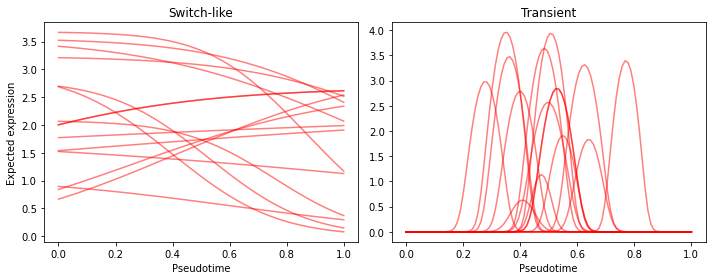
What does the model think the gene pseudotime curves look like before seeing any data? This can be quite informative to make sure our priors are in line with our prior knowledge. For this we can make use of prior predictive checks: We generate samples of the prior distributions of the parameters. One draw from each parameter gives us a set of parameters that come together to form one pseudotime curve. By drawing the curves of many parameter sets we get a rough idea of what the priors encode.

We thus sample 15 switch-like and 15 transient curves from the prior predictive:

with ouija:
    priorpred = pm.sample_prior_predictive()

fig, axs = plt.subplots(figsize=(10, 4), ncols=2, sharex=True)

xs = np.linspace(0, 1, 100)
sub = np.random.randint(0, 300, 15)

# Switch-like
ys = 2 * priorpred['peak_switch'][:, 0] / (1 + np.exp(-1 * priorpred['strength_switch'][:, 0] * (xs[:, None] - priorpred['time_switch'][:, 0]))) 
axs[0].plot(xs, np.log1p(ys[:, sub]), alpha=.5, c='r')
axs[0].set_xlabel('Pseudotime')
axs[0].set_ylabel('Expected expression')
axs[0].set_title('Switch-like')

# Transient
ys = 2 * priorpred['peak_transient'][:, 0] * np.exp(-1 * 10 * priorpred['length_transient'][:, 0] * np.square(xs[:, None] - priorpred['time_transient'][:, 0]))
axs[1].plot(xs, np.log1p(ys[:, sub]), alpha=.5, c='r')
axs[1].set_xlabel('Pseudotime')
axs[1].set_title('Transient')

fig.tight_layout()

We see that the priors on the parameters of the switch-like genes allow for both activiation as well as deactivation with varying levels of activation strength (though mostly diffuse), centered at various location on the pseudotime axis (though centered in the middle). The curves of the transiently activated genes have a strong prior belief that the activation happens at the center of the trajectory (recall $p \sim TruncNorm_{[0, 1)}(0.5, 0.1)$), with short activation times.

Before we move on to training the model, one thing must be addressed about the code above. The method pm.sample_prior_predictive convinietnlyl generates samples for us and returns a dictionairy with the samples for each parameter. What we wish to plot are not parameters however, but rather a set of parameters that we transform into gene expression values on a grid of points between 0 and 1. To make PyMC save such “intermediate” parameters, we can make use of the pm.Deterministic class, as indeed we have done (L15 of the 4th code block in the section Ouija in PyMC3).

However, where we wish to get samples of these deterministic “parameters” on a fixed set of pseudotime values, the PyMC model is defined to have the pseudotime values as parameters, which are sampled from as well. How do we tell PyMC to fix the values of the pseudotime parameter when we do prior predictive checks? One potential way is to set our grid of points as strong informative priors, though this still makes the pseudotime values non-determinstic. Instead, we will make a second model, where the pseudotime parameter $t$ is instead a pm.Data instance, which we can manipulate the values of after declaring the model. We will see that this also comes in handy when we do posterior predictive checks.

To avoid code duplication we build a model factory:

def build_model(pseudotimes=None):
    with pm.Model() as ouija:
        if pseudotimes is None:
            t = pm.TruncatedNormal('t', 
                priors['pseudotime_means'],
                priors['pseudotime_stds'],
                lower=0, upper=1, shape=N)
        else:
            t = pm.Data('t', pseudotimes)
        ... # Rest of the model
    return ouija

We can now build a seperate model for the purpose of predictive checking:

xs = np.linspace(0, 1, 100)
ouija_predictive = build_model(pseudotimes=xs)
with ouija_predictive:
    priorpred = pm.sample_prior_predictive(['mu_switch', 'mu_transient'])

fig, axs = plt.subplots(figsize=(10, 4), ncols=2, sharex=True)
sub = np.random.randint(0, 300, 15)

# Switch-like
axs[0].plot(xs, priorpred['mu_switch'][sub, :, 0].T, alpha=.5, c='r')
axs[0].set_xlabel('Pseudotime')
axs[0].set_ylabel('Expected expression')
axs[0].set_title('Switch-like')

# Transient
axs[1].plot(xs, priorpred['mu_transient'][sub, :, 0].T, alpha=.5, c='r')
axs[1].set_xlabel('Pseudotime')
axs[1].set_title('Transient')

Much better :-)

Identifiability

Before training the model, another issue must be addressed, namely that of model identifiability. When all genes have uninformative pseudotime priors, the likelihood of a particular ordering of the cells is equal to the reverse ordering, i.e. pseudotime == 1 - pseudotime from the model’s point of view. The consequence of this is a multi-modal posterior, where in this case we have two modes centered at the set of parameters that encode the best ordering and its inverse. When training the model using MCMC, each chain will only be able to explore one mode without being able to jump to the other mode. Ideally we’d like to train the model with multiple chains in order to evaluate our model fit. However due to this identifiability problem our chains are not guarenteed to converge to the same posterior mode (label switching). See here for a detailed analysis of this problem in the context of mixture models.

Informative priors can be incredibly helpful here. If we know that a gene is activated early, and we encode this in the activation parameter $t^{0}$ by shifting the mean to the left, then the ordering and its inverse are no longer as likely. Similarly, if we have collected the cells at different time points, then we can assign a prior ordering directly on the pseudotime parameters t.

As an alternative to setting informed priors, we can specify a common starting point for all MCMC chains as a way to encourage the chains the explore the same posterior region. Ouija uses this idea by taking the first principal component of the switching genes and using that as a starting point for the pseudotime parameter of each chain.

Here I simply fit the model with one chain to avoid dealing with the problem all together.

Inference

Finally let’s train the model on some data. For this we use the simulated data provided by Ouija in order to do a direct comparison with the Ouija vignette. The dataset contains 9 switch-like and 2 transiently activated genes. The simulation algorithm is specified in the supplementary of the Ouija paper. ¹ My PyMC code where I fit the model on this data can be found in the notebook here.

After fitting I wish to reproduce the following figure from the vignette:

Here the expression of each gene is plotted against the mean posterior pseudotime of the cells. The red line is the posterior mean gene expression for a evenly-spaced grid of pseudotimes values from 0 to 1. This is the same idea as the prior predictive plots shown before, but now the parameters are sampled from the posterior rather than the prior (posterior predictive checks). The code should therefore look familiar:

with ouija_predictive:
    postpred = pm.fast_sample_posterior_predictive(trace, 
                                var_names=['mu_switch', 'mu_transient'])

fig, axs = plt.subplots(figsize=(12, 13), ncols=2, nrows=6, sharex=True)

for p in range(P_switch):
    ax = axs.flatten()[p]
    ax.scatter(trace['t'].mean(0), np.log1p(Y_switch.iloc[:, p]), alpha=0.5)
    az.plot_hdi(xs, np.log1p(postpred['mu_switch'][:, :, p]), color='r', ax=ax)
    ax.set_title(Y_switch.columns[p])
    
for p in range(P_transient):
    ax = axs.flatten()[P_switch + p]
    ax.scatter(trace['t'].mean(0), np.log1p(Y_transient.iloc[:, p]), alpha=0.5)
    az.plot_hdi(xs, np.log1p(postpred['mu_transient'][:, :, p]), color='r', ax=ax)
    ax.set_title(Y_transient.columns[p])

fig.tight_layout()

Almost identical! A small difference is that I plot the highest density interval (HDI, L10+L16) rather than just the mean in order to show uncertainty.

Let’s also look at the inferred overdispersion. Recall that Ouija models the variance with a parametric form that depends on the mean: $\sigma_{ng}^2 = (1 + \phi)\mu_{ng} = \mu_{ng} + \phi\mu_{ng}$. The overdispersion parameter $\phi$ thus adds additional variance that cannot be explained by setting the variance equal to the mean. Let’s plot the prior and posterior of this parameter, as well as the mean-variance relationship.

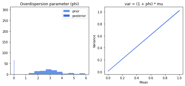
There is strong evidence that there is no overdispersion.

Another interesting aspect of the model is the dropout rate, which is modeled as a bernoulli regression model with the mean expression as a covariate (L3 of $\eqref{eq:noisemodel}$). Let’s do the same thing here.

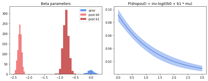
There is strong negative association between mean expression and dropout rate. And this makes sense, as we observe higher dropout right when cellular rna content of a gene is low. Of note is that the prior looks inadequate: Posteriors of both intercept and slope are outside the high probability region of the prior.

Posterior predictive checks

Does the model fit the data well? We already did a posterior predictive check in the previous section where we viewed the pseudotime curves per gene. Let’s do another one, but now visualizing the pseudotime curves over 2-dimensional PCA space. We will first project the data to two dimensions using PCA. We then generate a bunch of “fake” cells along the pseudotime axis, and map them to the same space using the trained PCA model. Per parameter set we get a unique curve and the variability between the curves should tell us about how uncertain the model is about the fit. Because we know the pseudotime value of each generated cell, we can color these pseudotime curves to get a feeling of how fast the cells move along the trajectory.

First the PCA plot. We color the cells by the pseudotime MAP.

Then we generate the cells and map their pseudotime curves to the trained PCA space. The code can be found in the method plot_curve_embedding here.

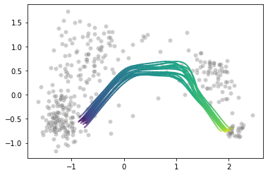
Pretty. Of note is that I didn’t generate the points from the likelihood, where most of the sampling variability will be. I will now make a plot where I pass the generated cells through the likelihood at five points along the pseudotime axis, and plot their densities again in PCA space. Code can be found in the method plot_predictive.

Conclusion

I have re-implemented Ouija in PyMC3 and shown that it reproduces the parameters shown in the vignette. Ouija provides an additional set of tools to interpret these parameters, such as statistical tests to determine order of activation of the genes, and clustering of the cells into metastable groups. The authors have also shown that the model can be fit using variational inference that comes for free with Stan. It might be interesting to try out PyMC’s VI sometime as well.

---

1. Campbell, K. R., & Yau, C. (2018). A descriptive marker gene approach to single-cell pseudotime inference. 10. ↩ ↩² ↩³

2. Townes, F. W., Hicks, S. C., Aryee, M. J., & Irizarry, R. A. (2019). Feature selection and dimension reduction for single-cell RNA-Seq based on a multinomial model. Genome Biology, 20(1), 295. https://doi.org/10.1186/s13059-019-1861-6 ↩

3. Svensson, V. (2019). Droplet scRNA-seq is not zero-inflated. BioRxiv, 582064. https://doi.org/10.1101/582064 ↩